Summary:

In this work, we continue our work about time series of yield difference of indices. Since last work result we decide to turn our focus on the yield difference between SSE50 and CSI500.

In the work, we at first refresh our strategy performance results with newest data, the data of the end of Aug. and Sep. then we reconsider our strategy execution and now the trading results are based on more directly tradable assets, ETFs. We would also consider the economic implications of our selected factors.

1. Indices introduction

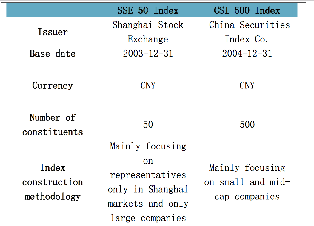
The SSE50 index is based on the scientific and objective method to select the 50 most representative stocks in the Shanghai securities market, which are the largest and abundant in liquidity. The intention of the index is to comprehensively reflect the overall situation by a group of leading enterprises with the most market influence in the Shanghai securities market. The SSE50 index has been officially released since January 2, 2004. The goal is to set up an investment index that is active, large and can be a base for derivative instruments.

CSI Small-cap 500 index (CSI500) is one of the index developed by the China Securities Index Co. The stock in the sample space is made up of 500 remaining largest stocks in the total A shares after dropping the top 300 stocks in the total market value or the components of CSI 300 index. The index comprehensively reflects performance of a group of small and medium market capitalization companies in A shares.

Table 1: Summary of the 2 indices.

2. Indices yield difference.

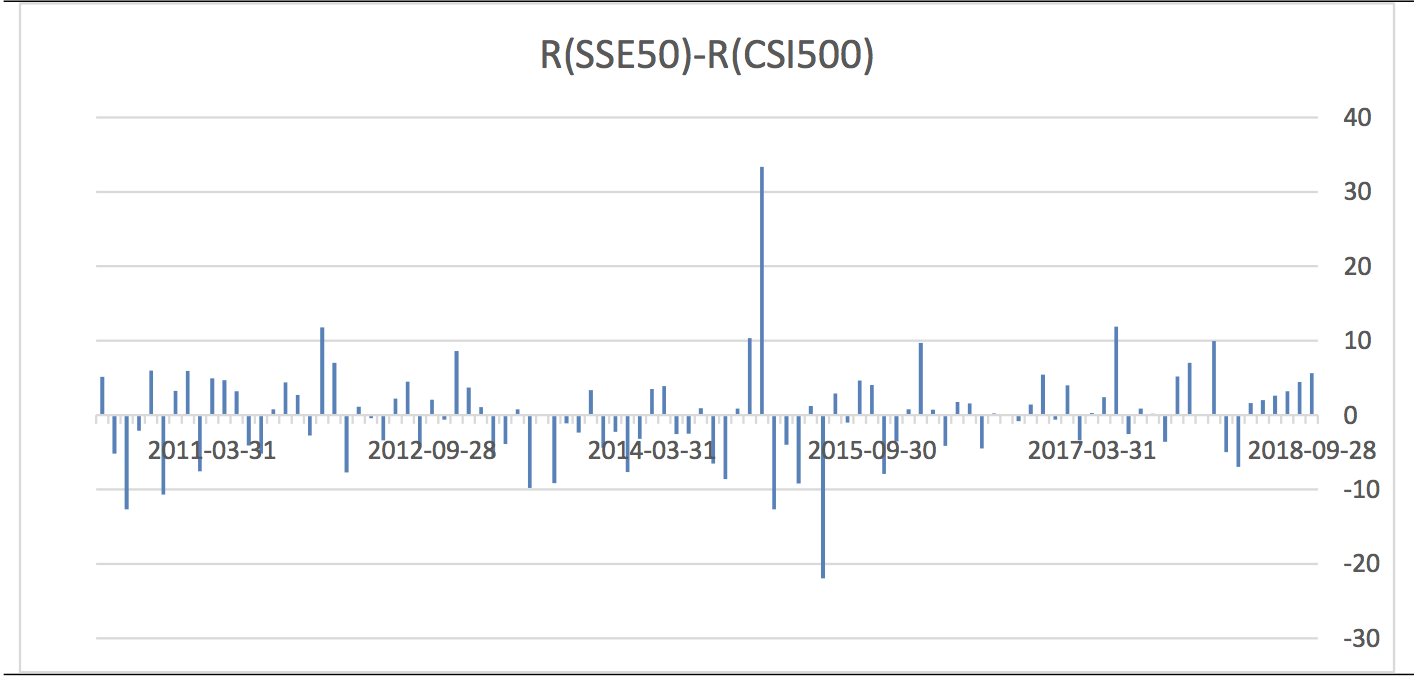
We observe yield difference of indices, we mainly focus on R(SSE50)-R(CSI500) and try to find whether such difference is predictable or there is such strategy that making superior performance.

In this work, we focus on monthly difference, we choose a time period of 100 months up to 2018/9/30 (Actually, just slightly different from our previous work).

Graph 1: Monthly R(SSE50)-R(CSI500) Time Series (%)

3. Last Work Performance Update

Input data including ratios between SSE50’s and CSI500’s P/E(TTM), ln(P/B(TTM)), P/S(TTM), P/CFO(TTM), CFO/E(TTM), Dividend Yield (TTM) and difference between SSE50’s and CSI500’s ROE(TTM), our consideration is developing strategy by setting P=60.

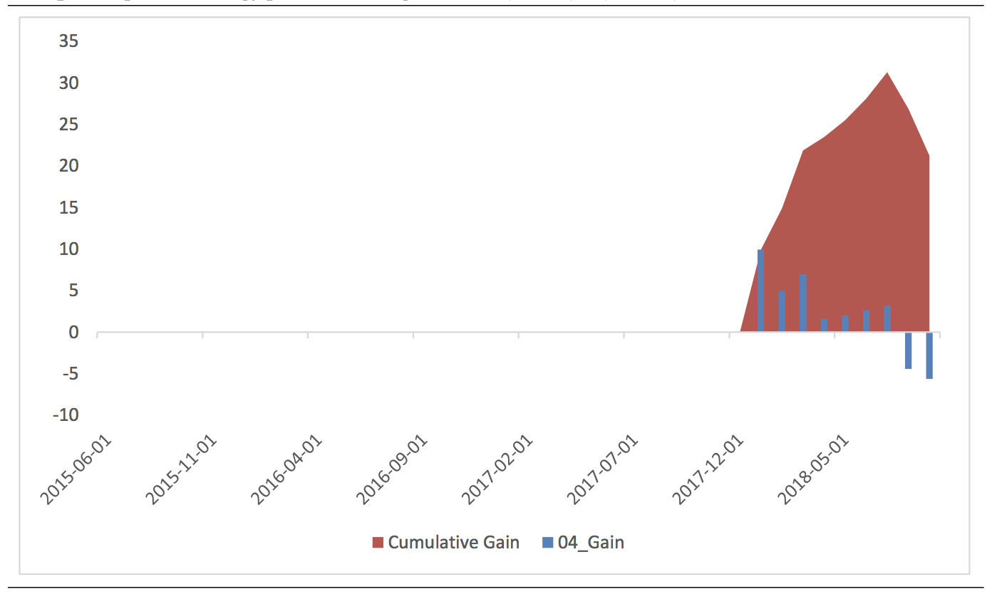
With the newest data, now we can review the performance of our strategy suggested in our last work (with P=60). Up to the time of 2018/9/28 our strategy had still selected a predictive relation with PE, ln(PB), PS, Div as independent variables for Aug and Sep, with p-values of F statistic 0.0127 and 0.0123 for the end Aug and July respectively . It made prediction that CSI500 would do better for Aug. and Sep. and that was false. Unfortunately, the strategy come with loss of -4.43% and -5.63% respectively and then the cumulative gain now is just 21.22%.

Graph 2: Updated Strategy performance regarded to R(SSE50)-R(CSI500) Time Series with P=60

4. With real word transaction condition.

In previous works, we consider trading execution by simply assuming trading directly on index values. However, it is not quite realistic. We would like to slightly change our work by assuming trading on relevant index ETFs, that is, 50ETF and 500ETF。It is worth to note that stock index values should be considered as accurate measures and reference, but ETF values should have some tracking error. Thus, when find predictive relation, we use index values (R(SSE50)-R(CSI500)), when we assume executing transactions, we use ETF values (R(50ETF)- R(500ETF)).

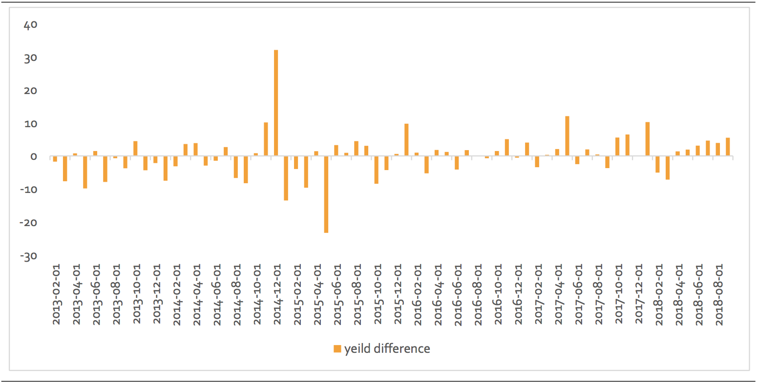
With newest data, the results are presented in the following graphs. Obviously, Graph 3 should be similar to Graph 1. However, 500ETF just listed since 2013, so there are less data points in Graph 3, but it would not be a problem as the earliest time we consider trading is in2015, with 100-month data and P=60.

Graph 3: Monthly R(50ETF)-R(500ETF) Time Series (%)

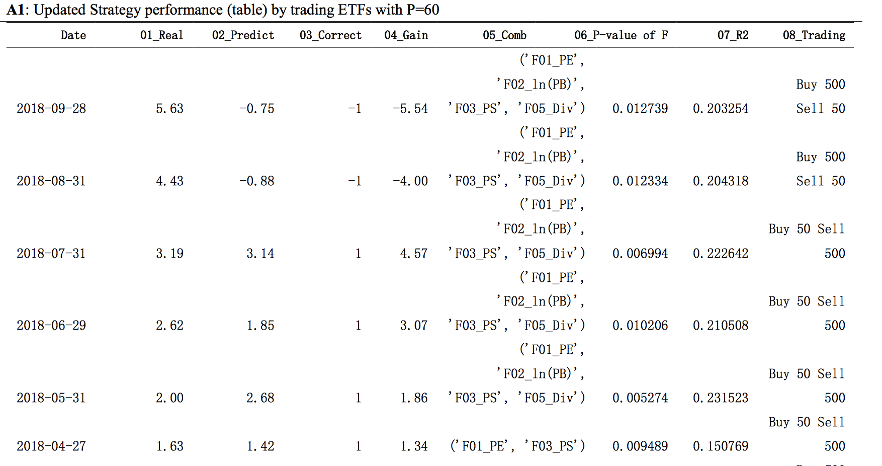
Graph 4: Updated Strategy performance by trading ETFs with P=60

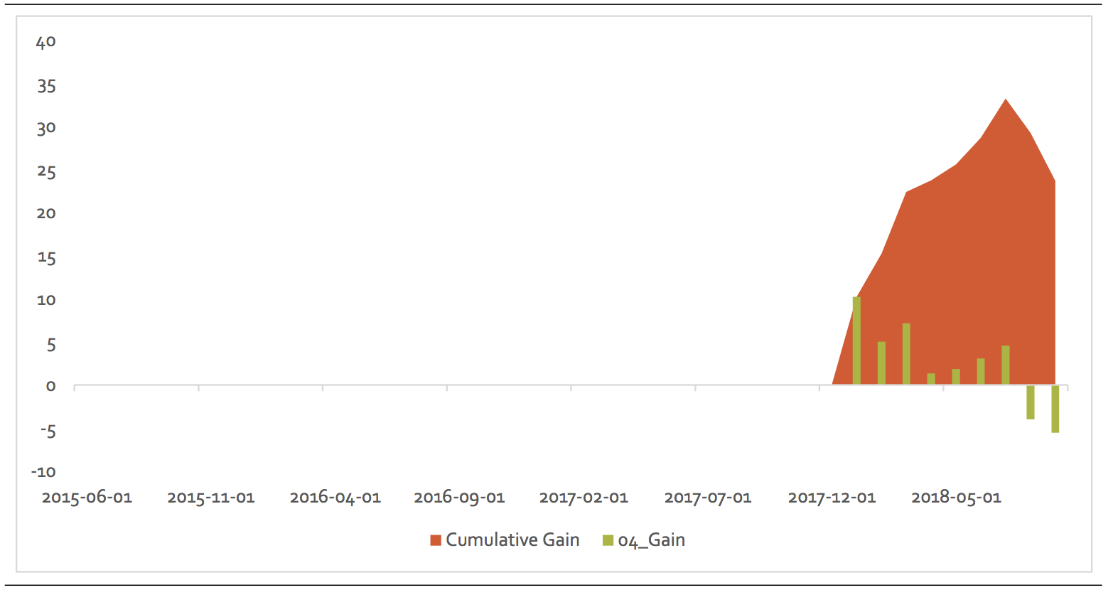
We also add a transaction expense assumption. For each time there are transactions assumed, there is a cost of 0.05%

The results end up with cumulative payoff of 23.68%, better than directly assuming trading on index values.

With the newest set factor data (2018/9/28), the strategy predicted that R(SSE50)-R(CSI300) =-2.01%, or CSI500 would do better than SSE50 in Oct. It still use the combination of PE, ln(PB), PS, Div) as independent variables.

5. Strategy Introduction

We rewrite our strategy introduction by adding the consideration of trading issue.

The logics is based on that a predictive relationship between the yield difference and factors may be not stable over long time, as the environment of the market keeps changing. However, it may be effective during a limited period if relations are so significant. That is, if we find some predictive relationship by observing data over period from T1 to T2, then this relation may exist over period T2 to T2+dT.

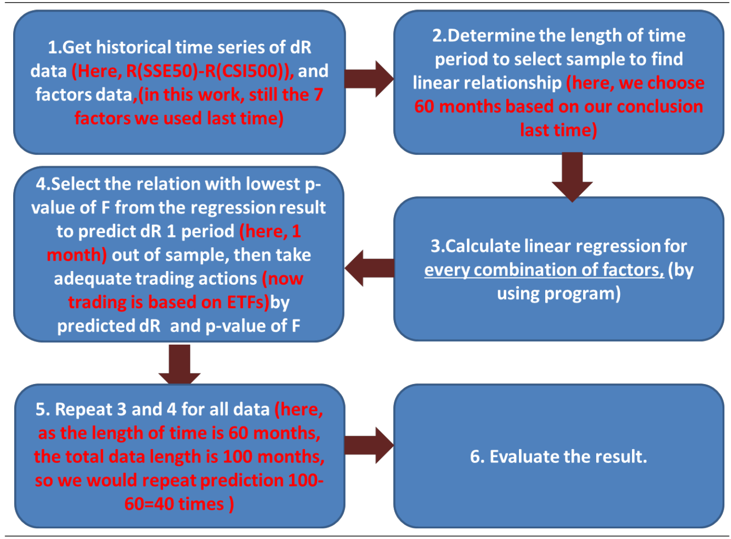
So, the strategy is, find the best predictive relation (the one with the lowest p-value of F) during T1=(T-1-P) to T2=(T-1), from regression results for all combinations of factors. If its p-value of F is below 0.05, then use this relationship to predict the indices yield difference, dR, at T (making out of ample prediction), then trade by the predicted result (long one’s ETF and short the other’s ETF). If the best predictive relation’s p-value of F is above 0.05, do nothing.

Graph 5: Strategy logics

6. Economic Implication of the model.

With 2018/9/28 data, the model, had selected the factors combination, PE, ln(PB), PS, Div, for 6 times. The regression parameters are similar among the 6 times. 111.81, -22.27, -50.33, 4.41 respectively for the 4 factors. So, in the predictively relation, PE, Div are positively related to yield difference while ln(PB), PS are negatively related and such relation is consistent through the strategy back test (with P=60, though detail number changed over time roll new data in old data out).

Note that the 4 factor values are calculated by the ratio of SSE50 and CSI500.

Negative regression parameters for PS, PB indicates that one with lower values of the 2 factors would tend to have better performance. That is, if SSE50 have less PS or ln(PB), the factors (by ratio of SSE50 and CSI500) tend to be less, then yield difference (R(SSE50)-R(CSI500)) tend to be high, SSE50 would have better performance than CSI500. Such 2 relations we think its reasonable, as lower PS, ln(PB) (or PB) indicates better valuations. We think it is reasonable to view that one with more attractive valuation level should perform better.

Positive regression parameters for PE, Div indicates that one with higher values of the 2 factors would tend to have better performance. As for Div, higher dividend payment is desirable for investors so a positive regression parameter for Div seems reasonable. But in the case of PE, high PE indicates less attractiveness in valuation but better prospect in growth. Assuming price is followed by a dividend discount model and then PE=1/(r-g). Higher PE indicate higher growth, which indicates higher price rising in next term. That is, if the price is fair, growth rate is accurately reflected in the price, then the one with higher PE should have better price performance in next term. In our case, index is likely to be fairly priced at most times, then it is possible that regression parameter for PE is positive.

Appendix:

摘要:

本报告将延续指数收益率差的考察，关注焦点仍为上次报告中注重的 R(SSE50)-R(CSI500). 这次我们首先将更新上次提出的策略表现结果，其数据至 2018/9/30。另外我们将会重新评估策略执行条件，

策略交易结果将基于实际指数 ETF 交易，另外我们也将探讨策略筛选出的预测关系的经济意义。

1. 指数介绍

上证 50 指数是基于科学和客观的方法选择上海证券市场中 50 大最具代表性的股票，它们是流动性最 大、流动性最强的股票。该指数的目的是综合反映上海证券市场最具市场影响力的一批龙头企业的整体情 况。SSE50 指数自 2004 年 1 月 2 日正式发布。目标是建立一个活跃的投资指数，可以作为衍生工具的标 的。

中证 500 指数(CSI500)是中国证券指数公司制定的指数之一，样本空间中的股票是在剔除沪深 300 指数后由总市值最大的 500 个的剩余市值最大的股票构成的。该指数综合反映了 A 股中小市值公司的业 绩。.

Table 1: Summary of the 2 indices.

2. 指数收益率差.

我们观察指数的收益率差异，在本次研究中我们主要关注在 R(SSE50)-R(CSI500)，并试图检验这种

收益率差异是否可预测，有无相应策略赚取超额收益。

在本次研究中， 我们专注于月收益率差，我们选择了一个 100 个月至 2018/9/30 的时间段(较上次的报告

后移2个月)

Graph 1: Monthly R(SSE50)-R(CSI500) Time Series (%)

3. 策略表现结果数据更新

输入数据包括 SSE50 和 CSI500 的 P/E(TTM)、Ln(P/B(TTM))、P/S(TTM)、P/CFO(TTM)、 CFO/E(TTM)、股息收益率(TTM)之间的商和 SSE50 和 CSI500 的 ROE(TTM)之间的差。另根据上 一次结论，我们选定 P=60

根据最新数据，我峨嵋年回顾了上次提出策略的表现。截至 2018/9/28，我们的策略连续 2 个月选取了 基于 PE, ln(PB), PS, Div 因子作为模型自变量，预测回归 F 统计量的 p 值在七月底和八月底 0.0123 和 0.0127。 策略预计 CSI500 表现在八月九月将优于 SSE50。然而该预测是错误的，在八月与九月分别造成了-4.43%和 -5.63%的损失，因此近累计收益降为 21.22%

Graph 2: Updated Strategy performance regarded to R(SSE50)-R(CSI500) Time Series with P=60

4. 考虑实际交易情况.

在以前的报告中，我们简单假定了直接交易指数。然而，交易指数斌并不是非常现实，因此我我们将 稍微改变一下结果的计算方式，策略执行将基于与指数对应的 ETF，即 50ETF 和 500ETF。值得注意的是 指数能准确反映个表组合的价格但 ETF 有跟踪误差。因此在寻找预测关系时，我们仍然使用指数值和收益 率差。

结合最新数据，结果在下面 2 图呈现。显然图 3，图 1 应当相似。然而 500ETF2013 年才发布，所以图 3 数据点较少。鉴于我们从 2015 才考虑交易，这不会影响我们的计算。

Graph 3: Monthly R(50ETF)-R(500ETF) Time Series (%)

Graph 4: Updated Strategy performance by trading ETFs with P=60

我们也增加了一个交易成本假定。每一次有交易执行的时候，每个 ETF 将有一个 0.05%的交易成本

更换为 ETF 为交易标的后，策略累计收益变为 23.68%，较直接交易指数值略有提高。

根据最新的因子数据(2018/9/28), 我们的策略预计 R(SSE50)-R(CSI300) =-2.01%，或说在 10 月 CSI500 较 SSE50 表现更好。预测关系仍然基于 PE, ln(PB), PS, Div 这 4 个因子为自变量

5. 策略介绍 在考虑交易情况后我们重写了策略的运行逻辑。

由于市场环境不断变化，指数收益率差与因子间的预测关系长期来看是不稳定的。然而，这种关系，若是 显著，很可能在样本外的有限时间内仍然成立。也就是说，若我们发现了在 T1 至 T2 期间存在某个显著的预 测关系，该关系也许在 T2 至 T2+dT 时间段也存在。

所以我们将考虑这样一个策略，在 T1=(T-1-P)至 T2=T-1 的时间段内从所有回归组合中找出线性预测能 力最显著的关系(有最小 F 统计量 p 值)，且 F 统计量 p 值小于 0.05，用该关系来预测 T 时刻指数收益率差 dR(即样本外预测)，然后根据预测结果执行交易。当然最显著的关系的 F 统计量 p 值若大于 0.05，则不做 交易。

Graph 5: Strategy logics

6. 模型经济意义.

根据 2018/9/28 数据，我们的模型已经连续选择 PE, ln(PB), PS, Div 四个因子组合 6 次。回归结果的参数较 为接近，111.81, -22.27, -50.33, 4.41。因此，在预测关系中 PE, Div 因子与收益率差正相关，而 ln(PB), PS 与收 益率差负相关。该规律在 P=60 的情况下保持不变。

考虑到 4 个因子均为 SSE50 与 CSI500 相应指标之比。

PS, PB 负的回归参数表明指数有较低 PS 或 PB 的将趋向于有较好表现。如 SSE50，PS，ln(PB)较小，相 应因子(由 SSE50 与 CSI500 相应指标比值算出)将较小，则收益率差(R(SSE50)-R(CSI500))趋向于较高，即 SSE50 将有较好表现。我们认为这个关系是解释的通的，较低的 PS，PB 反映更好的估值。估值较低的其表现 较好。

正回归参数的 PE，Div 表明，一个具有较高值的两个因素将倾向于具有更好的表现。对于 Div 而言，股利 支付对投资者更为有利，因此DIV的正回归参数似乎是合理的。但在PE的情况下，高PE表现出较低的估值， 但更好的增长前景。假设价格由股利贴现模型解释，然后 PE=1/ (r-g)。较高的 PE 显示了较高的增长率， 这意味着下一个月的价格将上涨较快。也就是说，如果价格是公平的，增长率准确地反映在价格中，那么 PE 值较高的公司应该在下一期有更好的价格表现。在我们的情况下，指数很可能在大多数时候是合理定价的，那 么 PE 的回归参数为正是可能的。

Copyright by fangquant.com